Roadster engineering 02: power or grip for a one-second launch?Roadster 技术拆解 02：一秒加速，先补功率还是抓地力？

Put the target beside the limits先把目标与限制放在一起

An extra 25% of usable drive power sounds like an obvious upgrade. In the example below, it does not shorten the launch at all: the tyres are already the limiting element. A larger reduction ratio has the same result. The useful design question is which limit must move first, and what becomes the next constraint.可用电驱功率增加 25%，看起来是很直接的升级。但在下面的示例中，它完全没有缩短起步用时：轮胎已经先到极限。加大减速比，结果也一样。真正需要回答的是：先移动哪一条限制，之后又会被什么卡住。

Start with the target from Part 1’s launch calculation: rest to 60 mph in one second, without rollout. For this installment, choose an illustrative 2,000 kg vehicle. Specify constant acceleration for this target: the required forward force is 53.6 kN, from mass times acceleration. Before selecting a battery or motor, compare that requirement with the force each part of the system can support.从第一期的起步目标继续：从静止到 60 mph，用时一秒，不扣除起步距离。本期取一辆假设质量为 2,000 kg 的车。先规定这条目标轨迹采用匀加速：质量乘以加速度，得到所需前向力 53.6 kN。挑电池和电机之前，先把这项要求与系统各环节能支持的力放在一起。

All numerical hardware values below are explicit model assumptions, not Roadster specifications or test results. Tesla’s Roadster reservation agreement, checked 18 October 2026, still describes a vehicle under development. The calculations do not presume its motor type, pack voltage, cell layout or gear ratios.下文硬件数值均为明确给定的模型假设，不是 Roadster 规格或实测结果。2026-10-18 核对的 Tesla Roadster 预订协议仍将车辆描述为开发中；本文不预设它的电机类型、电池电压、电芯排列或减速比。

The same model gives a useful counterexample: a gear change alone saves no time, but adding constant downforce and then changing the ratio cuts the idealized time from 1.823 to 1.464 s. The gear boundary, cost allowance and one-second feasibility map below show where that conclusion holds, what costs erase it, and which capacities must change together.同一个模型里，单改齿比没有收益；增加恒定下压力后再改齿比，理想化用时却从 1.823 降至 1.464 秒。后面的齿比边界、代价预算与一秒可行域分别回答：结论在什么范围成立，哪些代价会抵消收益，以及哪些能力必须一起改变。

The lowest ceiling decides真正起作用的是最低的那条上限

Use one baseline throughout: 2,000 kg, tyre coefficient μ = 1.5, aggregate motor torque 1,200 N·m, reduction ratio G = 9, rolling radius 0.34 m and 903.07 kW available wheel power. Assume all-wheel drive can use the whole-vehicle grip limit, with no additional downforce. Torque sets one force ceiling, grip another; the power ceiling falls with speed because force equals power divided by speed. The car can use only the lowest of the three.先固定同一组基线：质量 2,000 kg，轮胎附着系数 μ = 1.5，等效电机总转矩 1,200 N·m，减速比 G = 9，滚动半径 0.34 m，可用轮端功率 903.07 kW；假设全轮驱动能够利用整车抓地力，没有额外下压力。转矩和抓地力分别给出一条力的上限；功率对应的力则随车速下降，因为力等于功率除以速度。车真正能用上的，是三者中最低的一项。

The target requires 53.6 kN throughout the interval; the baseline can use only 29.43 kN. At 60 mph, the torque and power ceilings are also below the target, at 30.81 and 33.67 kN. Raising grip alone therefore cannot meet this trajectory either. First follow how the electrical and mechanical ceilings arise; then compare which changes actually reduce the model’s elapsed time.目标在整段过程中需要 53.6 kN，基线却只能用到 29.43 kN。到 60 mph 时，转矩与功率对应的上限分别为 30.81 和 33.67 kN，也都低于目标。因此，单独补抓地力同样达不到这条轨迹。先沿电驱链说明这些上限从哪里来，再比较哪些改动确实能缩短模型用时。

Little energy, a demanding delivery rate能量账单不大，交付速度却很苛刻

The energy and average power depend on the endpoints and elapsed time. The 1.44 MW endpoint value additionally assumes constant acceleration: force stays constant while speed rises, so rises with it. These figures exclude air resistance, rolling resistance, rotating parts and conversion losses. Here the tyres supply all propulsion; direct jet thrust would change the wheel-drive requirement.能量与平均功率由起终状态和用时决定；1.44 MW 的终点功率还依赖匀加速这一假设：力保持不变，速度不断升高，因此 也随之升高。这里未计空气阻力、滚阻、旋转部件和能量转换损失，并且假设推进全靠轮胎；如果喷流直接推动车身，轮端所需功率就会改变。

This is why adding kWh cannot, by itself, solve a launch problem. Energy describes how much can be delivered in total; power describes its delivery rate. MIT EV Team’s battery specification guide makes the corresponding distinction between capacity, energy, current and power ratings.因此，增加多少 kWh，并不能单独回答起步能否更快。能量描述总共能交付多少，功率描述交付得有多快。MIT 电动车团队的电池规格指南区分了容量、能量、电流和功率这些不同的指标。

Follow the power, including what becomes heat沿功率往前走，也追踪变成热的部分

The battery supplies DC electrical power. The inverter switches that supply to control motor winding currents; the motor turns electrical input into shaft torque and rotation. A reduction gear trades shaft speed for wheel torque. This division of work is described in the U.S. Department of Energy’s electric-vehicle component overview. Every stage has a limit, and every lossy stage leaves less power for the next one.电池提供直流电功率，逆变器通过开关控制电机绕组中的电流，电机把电能转换成轴上的转矩与转动，减速器再用转速换取轮端转矩。美国能源部的纯电动车部件说明给出了这些部件的分工。每一段都有自己的上限，存在损耗的环节也会让下一段能拿到的功率减少。

1. Battery terminals电池端口1,000 kW

   DC input to the drive送入电驱的直流功率

2. Inverter output逆变器输出980 kW

   98% · 20 kW lost效率 98% · 损耗 20 kW

3. Motor shafts电机轴端931 kW

   95% · 49 kW lost效率 95% · 损耗 49 kW

4. Wheel shafts轮端903 kW

   97% · 27.9 kW lost效率 97% · 损耗 27.9 kW

Voltage is measured in volts, current in amperes, torque in N·m and angular speed in rad/s. The efficiency factors are fractions of power retained. Real efficiencies vary with current, speed and temperature; fixed values here keep the accounting visible. They are unsuitable for predicting a whole drive cycle or standstill heating.电压用伏特，电流用安培，转矩用 N·m，角速度用 rad/s；各个效率系数表示保留下来的功率比例。真实效率随电流、转速和温度变化，这里固定取值，是为了看清功率如何分配，不能用来预测完整工况的能耗或堵转发热。

The battery has to hold its voltage under load电池必须在大电流下撑住电压

A pack that stores enough energy may still fail the power requirement. Drawing current lowers its terminal voltage and generates heat. A simple open-circuit voltage plus resistance model makes the coupling explicit; MathWorks’ battery equivalent-circuit documentation shows the fuller model, including dynamic polarization and additional heat terms.总能量足够，电池仍可能过不了功率这一关。电流流出时，端电压会下降，也会产生热。用开路电压加内阻的简化模型，就能看出两者如何耦合；MathWorks 电池等效电路文档还包含动态极化及其他热量项。

Here resistance is an approximation for a specified state and timescale, not a permanent pack constant. State of charge, temperature, minimum cell voltage, current limits and pulse duration all matter. A useful specification therefore says how much power is available, for how long, and from which starting conditions. The Battery Power Estimator equations explicitly combine voltage, current, state of charge and a prediction interval.这里的内阻只是特定状态和时间尺度下的近似，并非电池包永远不变的常数。荷电状态、温度、最低单体电压、电流上限和脉冲持续时间都会影响结果。因此，有用的规格必须说明：从什么初始状态出发，能提供多大功率，持续多久。电池可用功率估计器的公式就同时考虑了电压、电流、荷电状态和预测时间窗口。

Higher voltage does not erase cell heating提高电压，并没有消除电芯发热

At fixed power, doubling voltage halves pack current. A cable with unchanged resistance then produces one quarter of the resistive heat. But rearrange the same cells into twice as many series positions and half as many parallel branches: pack resistance becomes four times larger. Each cell still carries the same current. The cable benefit and the cell result are different calculations.相同功率下，电压翻倍，整包电流减半；如果一根电缆的电阻不变，它的电阻发热就降到四分之一。但若只是把同一批电芯改成两倍串联、半数并联，整包内阻会变成四倍，每颗电芯承受的电流仍然相同。电缆得到的好处，与电芯内部的结果，是两笔不同的账。

Separate wiring comparison: identical assumed 3.6 V, 5 Ah cells with 2 mΩ resistance and equal current sharing; s means series, p parallel. Currents use nominal voltage and ignore sag, so 360 kW is not the exact loaded terminal output. This is circuit accounting, not a cell safety rating. Higher voltage also changes insulation, switching-device and protection requirements.这是独立的接线对照：假设电芯均为 3.6 V、5 Ah、内阻 2 mΩ，支路均匀分流；s 表示串联，p 表示并联。电流按标称电压计算、忽略压降，因此 360 kW 不代表带载时精确的端口输出。它验证电路关系，不给出电芯的安全工作额定值。提高电压也会改变绝缘、开关器件和保护的要求。

Current makes torque; voltage makes room for speed电流建立转矩，电压为转速留下余量

The inverter does more than turn DC into AC. By switching the DC bus and using current feedback, it controls the magnitude and direction of the stator’s magnetic field relative to the rotor. That relationship produces torque. In a permanent-magnet motor example, field-oriented control separates a torque-producing current component from a flux-related component. Rotor saliency in an interior-permanent-magnet design also contributes reluctance torque. None of this identifies which motor Tesla will use.逆变器不只是把直流变成交流。它切换直流母线电压，并利用电流反馈，控制定子磁场相对转子的大小与方向，由这种关系产生转矩。以永磁电机为例，磁场定向控制把电流分成与转矩、磁通相关的分量；内嵌式永磁电机的转子磁阻在不同方向上存在差异，还能由此产生磁阻转矩。这里解释一种电机原理，不据此判断 Tesla 将使用哪种电机。

At low speed, winding current, inverter current and heat typically constrain torque. As speed rises, the motor’s back EMF rises too, leaving less voltage headroom for current control. Beyond a base speed, field weakening reduces the effective flux to keep operating within the voltage limit, while consuming part of the available current capability. TI’s IPMSM field-weakening and MTPA application note, sections 2.2–2.3, develops these current and voltage constraints.低速时，绕组电流、逆变器电流能力和发热通常限制了转矩。转速升高后，电机反电动势也随之增大，留给电流控制的电压余量变小。超过基速后，弱磁控制降低有效磁通，使运行仍满足电压限制，同时占用一部分可用电流能力。TI 的 IPMSM 弱磁与 MTPA 应用笔记第 2.2—2.3 节展开了这些电流与电压约束。

For the next calculation, replace these detailed limits with a constant-torque region followed by a constant-power region, ending at a maximum mechanical speed. It is a useful envelope, not a complete motor map. Real high-speed power can fall, and temperature or bus-voltage changes can move the boundaries.为了继续计算，下面把这些复杂限制近似成：先恒转矩，后恒功率，最后受最高机械转速限制。这个包络适合分析，但不是完整电机地图。真实电机在高转速下可能继续掉功率，温度和母线电压变化也会移动这些边界。

Two ceilings, one transition两个上限，一个转折

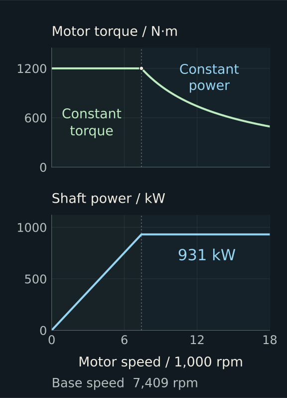
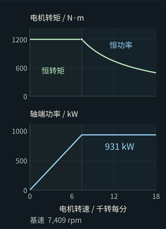
Assume an aggregate motor torque limit of 1,200 N·m and shaft-power limit of 931 kW. Their intersection gives a base speed of about 7,409 rpm.假设等效电机总转矩上限为 1,200 N·m，轴功率上限为 931 kW。两者相交，得到约 7,409 rpm 的基速。

Below it, more speed means more power at the same torque. Above it, twice the speed permits only half the torque if power is unchanged.基速以下，转矩不变，转得更快就能交付更多功率；基速以上，若功率不变，转速翻倍就只能保留一半转矩。

A gear multiplies torque, not power齿轮放大转矩，不放大功率

Define reduction ratio , and effective rolling radius . In this simple no-slip kinematic model, . The Simple Gear model expresses the corresponding speed and torque constraints. A larger ratio gives more wheel torque at the same motor torque, but reaches the same motor speed at a lower vehicle speed.定义减速比 ，轮胎有效滚动半径为 。在这里的无滑移运动学近似中， 。Simple Gear 模型给出了对应的转速与转矩约束。减速比更大，相同电机转矩能换来更大的轮端转矩，但电机会在更低的车速下达到同样的转速。

In the constant-power region, substituting the motor torque makes the gear ratio cancel: wheel force becomes wheel power divided by speed. More reduction cannot create additional power. It moves the torque-limited region and changes the speed range in which the motor can operate.进入恒功率区后，把电机转矩代入，减速比会消掉：轮端驱动力就是轮端功率除以车速。加大减速比不会凭空增加功率；它改变的是转矩受限的范围，以及电机能够覆盖的车速区间。

At zero speed use the finite torque-force limit, not division by zero. With a 0.34 m rolling radius, 97% gear efficiency and G = 9, the assumed motor supplies at most 30.8 kN before the power limit takes over. G = 12 raises that torque-based ceiling to 41.1 kN. Whether either increase accelerates the car depends on the tyres.零车速时直接使用有限的转矩换算力，不做除以零的计算。取滚动半径 0.34 m、齿轮效率 97%、G = 9，这台假设电机在功率限制介入前最多提供 30.8 kN；G = 12 则把转矩对应的力上限提高到 41.1 kN。但它能否让车更快，还要经过轮胎这一关。

Plot the force the car can actually use画出车真正能用上的力

For a straight-line comparison, add a constant grip ceiling of . Set μ = 1.5, g = 9.81 m/s² and m = 2,000 kg, giving 29.43 kN. Assume all-wheel traction can use this whole-vehicle ceiling. There is no suction, jet thrust, resistance or rotating inertia in this example. These assumptions deliberately isolate the powertrain–grip interaction.为了比较直线加速，再加入一个固定的抓地力上限 。取 μ = 1.5、g = 9.81 m/s²、m = 2,000 kg，得到 29.43 kN，并假设全轮驱动能够利用这项整车上限。本算例不含吸附、喷流、阻力和旋转惯量，用这些简化单独观察电驱与抓地力怎样相互限制。

Extra torque can disappear at the contact patch多出来的转矩，可能用不上

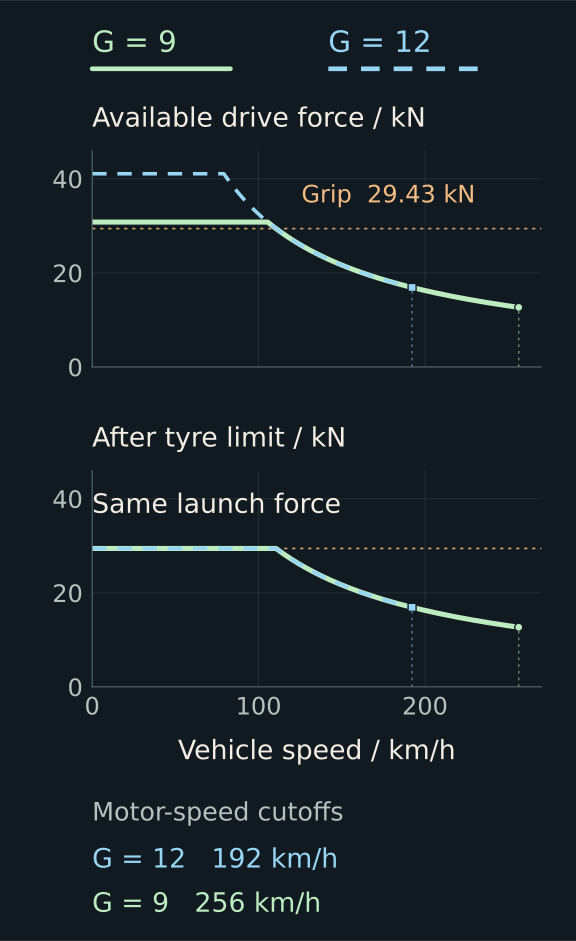
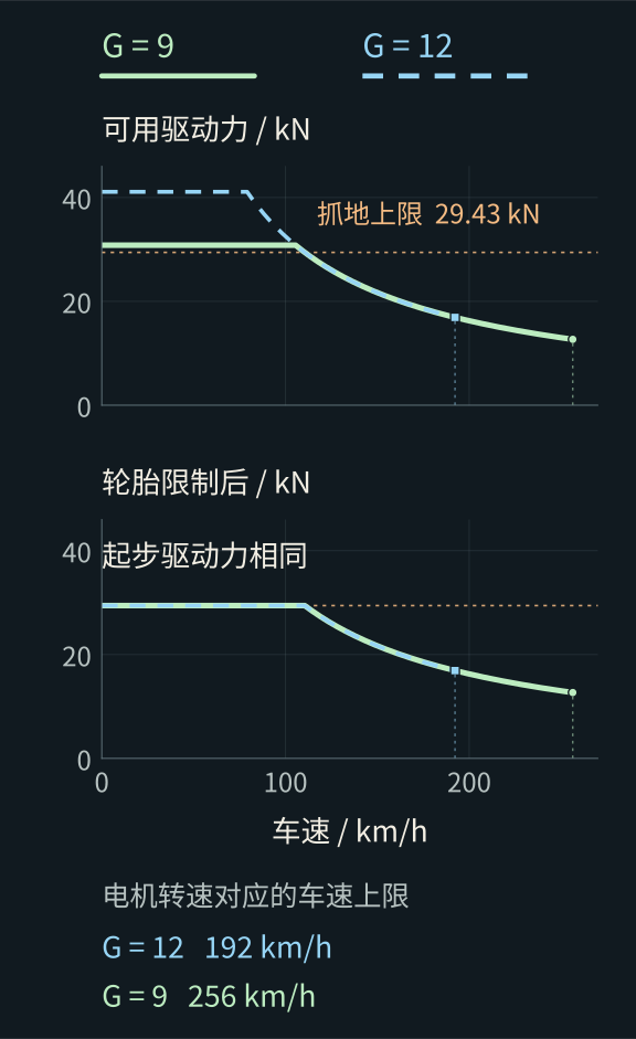
Both ratios already exceed the 29.43 kN grip ceiling at low speed. The higher ratio adds no usable launch force in this example. Both become power-limited at about 110.5 km/h.两个减速比在低速时都已超过 29.43 kN 的抓地力上限。因此，这个例子中更大的减速比并没有增加可用的起步力。两者约在 110.5 km/h 后转为功率受限。

At 150 km/h, both deliver about 21.7 kN. At 200 km/h, G = 9 still has a valid operating point; G = 12 would require more than 18,000 rpm and is outside the model’s allowed range.到 150 km/h，两者都能提供约 21.7 kN。到 200 km/h，G = 9 仍有有效工作点；G = 12 却要求超过 18,000 rpm，已经落在模型允许范围之外。

This also explains why more downforce is conditional. It helps where grip is the smallest term. Where electrical or mechanical power is already the smallest term, raising grip alone does nothing; a fan drawing from the same DC supply can reduce available drive power. That connects this envelope directly to Part 1’s fan-power tradeoff.这也解释了为什么增加下压力有条件：只有抓地力是最小项时，它才有用。如果最小项已经变成电功率或机械功率，单独提高抓地力不会增加驱动力；风扇若从同一个直流功率池取电，甚至会降低电驱可用功率。这正好接回第一期的风扇功耗取舍。

Four changes, one controlled comparison四种改动，用同一把尺子比较

The horizontal target line prescribes constant acceleration. To compare upgrades, instead let the model use its full available force at every speed; acceleration may vary. Integrate the time needed to reach 60 mph, with denoting the maximum usable force at that speed. This gives the shortest time within the stated, time-invariant model, with no rollout, control delay, resistance or rotating inertia. It is not a measured time or a Roadster prediction.前面的水平目标线规定了匀加速。比较升级方案时，改为让模型在每个车速都用满可用驱动力，允许加速度变化，再把达到 60 mph 所需的时间积分出来，式中 为该车速下的最大可用驱动力。这是给定、不随时间变化的模型内的最短用时：不扣除起步距离，不计控制延迟、阻力和旋转惯量；它不是实测成绩，也不是 Roadster 预测。

Each of the first four changes starts from the same baseline; changes are not cumulative. The power case raises the usable power ceiling of the whole drive chain by 25%, with torque, mass and efficiencies held fixed. The downforce case adds a constant 4,905 N from rest, with no power draw, drag or hardware mass: an optimistic isolated-force comparison. With downforce , replace the grip term with .前四项改动都从同一基线出发，不累加。功率方案把整条电驱链可交付的功率上限提高 25%，同时保持转矩、质量和效率不变。下压力方案从静止就额外提供恒定的 4,905 N，不计取电、阻力和装置质量，是只观察新增作用力的乐观对照。加入下压力 后，将抓地项改为 。

The zero gain from reducing mass is specific to while grip is the active limit. It does not extend to power-limited acceleration or to tyres with load-dependent friction. The load-dependent Magic Formula tyre model makes that missing dependence explicit. Likewise, a normal aerodynamic wing does not supply the assumed extra 4,905 N from rest: aerodynamic force depends on relative airspeed squared. A fan system would need its electrical draw and hardware mass restored to the calculation.减重没有收益，仅限于抓地力是有效限制、且 的情况，不能外推到功率受限的加速，也不能外推到摩擦特性随载荷变化的真实轮胎。采用载荷相关系数的 Magic Formula 轮胎模型明确包含了这一缺项。同样，普通气动翼并不能从静止起就提供这里假设的 4,905 N，因为气动力取决于相对气流速度的平方；若用风扇实现，则必须把取电和装置质量补回计算。

Change the grip budget, and the gear choice changes抓地条件改变后，减速比的选择也会改变

With downforce, the 36.79 kN grip ceiling is above G = 9’s torque-force ceiling. G = 12 can use that grip at low speed, then becomes power-limited at 88.4 km/h. A gear change that saved nothing on its own now matters. The gains cannot be added independently: one change creates room for the next. The lower motor-speed cutoff remains, and the unpriced downforce costs remain too.增加下压力后，36.79 kN 的抓地上限已经高于 G = 9 的转矩上限。G = 12 能在低速用上这份抓地力，随后在 88.4 km/h 转为功率受限。单独改齿比原本没有收益，现在却有了作用。收益不能独立相加：前一个改动给后一个改动腾出了空间。更低的电机转速车速上限仍然存在，下压力尚未计入的代价也仍然存在。

How far does the gear decision hold?齿比选择，在什么条件下改变？

“Keep G = 9” applies to the baseline, not every grip condition. With the same motor, its torque-derived wheel-force ceiling is 30.81 kN. With no added downforce, grip reaches this ceiling at μ ≈ 1.5704, only 4.7% above the assumed 1.50. Above that value, G = 9 cannot use all the available grip, and G = 12 starts to reduce the integrated launch time.“保留 G = 9”只适用于当前基线。沿用同一台电机，它的转矩换算力上限是 30.81 kN；没有额外下压力时，μ 达到约 1.5704，抓地力就碰到这条上限，只比假设的 1.50 高约 4.7%。超过这个值，G = 9 已用不满抓地力，G = 12 开始缩短积分用时。

At μ = 2 and 1 MW DC, the model gives 1.741 s for G = 9 and 1.383 s for G = 12. At low power, both spend more time on the same power-limited curve, so the gain becomes smaller; it is not exactly zero above the threshold. The higher ratio still sacrifices speed range. This map compares only the launch interval.例如 μ = 2、直流功率 1 MW 时，G = 9 为 1.741 秒，G = 12 为 1.383 秒。功率较低时，两者更早进入同一条功率受限曲线，齿比收益随之缩小，但在 μ 超过阈值后并非严格为零。更大的减速比仍会缩小车速覆盖范围；这张图只比较起步区间。

There are two other useful checks at the original μ = 1.5. Aggregate torque below about 1,146 N·m makes G = 9 torque-limited at launch. Available DC power below about 874 kW makes power intervene before 60 mph. These thresholds turn “recheck at another state” into measurable capacity requirements.回到原来的 μ = 1.5，还有两个可核查的门槛：等效电机总转矩低于约 1,146 N·m，G = 9 的起步就转为转矩受限；可用直流功率低于约 874 kW，功率限制会在 60 mph 之前介入。检查其他荷电状态或温度下的包络时，可以先核对这两项能力。

How much cost can downforce tolerate?下压力的收益，能承受多少代价？

Now restore two omitted costs to the 4,905 N downforce plus G = 12 case. Let added hardware mass be and constant auxiliary DC draw be . Keep the total pack-terminal ceiling at 1 MW: subtract auxiliary draw before drivetrain losses, and add the hardware mass to both inertia and tyre normal load. Compare the result with the original G = 9, no-downforce, 2,000 kg baseline.现在把两项省略的代价补回“4,905 N 下压力 + G = 12”方案。设新增装置质量为 ，恒定辅助直流功耗为 。电池端口总上限仍为 1 MW：先扣除辅助用电，再计算电驱损耗；新增质量同时计入惯性和轮胎法向载荷。比较基准始终是原来的 G = 9、无下压力、2,000 kg 车辆。

Use the same time integral with M in place of m. The boundary below is where the modified vehicle matches the baseline time of about 1.823 s: one side still improves the launch, and the other has spent away the benefit. Downforce is held at 4,905 N throughout; mass and auxiliary draw are independent imposed costs.沿用同一个时间积分，将质量换成 M。下图边界上的方案都与基线用时相同，约为 1.823 秒：一侧仍比基线快，另一侧已被新增代价抵消。下压力全过程固定为 4,905 N，质量与辅助功耗作为两项独立代价扫描。

With no added mass, the break-even auxiliary draw is about 454 kW; with 200 kg added, it falls to 391 kW. The limits cannot be spent independently. A more modest example, +100 kg and 100 kW auxiliary draw, gives 1.512 s, still below the 1.823 s baseline. Holding downforce fixed does not establish that a real device can deliver it at those costs: this chart applies only if the device sustains 4,905 N throughout. If measured downforce differs, recalculate the boundary before comparing its mass and electrical draw.不增加质量时，辅助功耗的收支平衡点约为 454 kW；增加 200 kg 后，降至约 391 kW。这两项额度不能独立用满。另取“增加 100 kg、辅助功耗 100 kW”的组合，模型得到 1.512 秒，仍快于 1.823 秒基线。但固定下压力的前提并未证明真实装置能以这些代价实现它；只有装置全过程提供 4,905 N 下压力时，才能直接用这张图核对质量与功耗。若实测下压力不同，需先重新计算边界。

Which force–power envelopes can reach one second?哪些力与功率的组合，能够达到一秒？

The opening used constant acceleration to make the requirement visible. The design question is broader: can the available force envelope reach 60 mph within one second, allowing acceleration to change? Keep the 2,000 kg mass and the same resistance-free, time-invariant model. Define C as the smaller of the grip and torque-derived force ceilings, and P as the available wheel-power ceiling.开头用匀加速把需求画成一条直线。设计判断可以更一般：允许加速度变化，可用的驱动力包络能否在一秒内到达 60 mph？仍取质量 2,000 kg，沿用不计阻力、边界不随时间变化的模型。用 C 表示抓地力与转矩换算力中较低的上限，P 表示可用轮端功率上限。

At rest use . The envelope is constant-force up to , then constant-power. Integrating those two pieces gives the same elapsed-time criterion used for all upgrade comparisons.静止时取 。先以恒定驱动力加速，到 后转入恒功率段。分别积分两段，就得到与所有升级对照一致的用时判据。

Write the elapsed time as . If , power never limits the launch, so the force stays at C:将积分用时记为 。当 时，功率限制尚未介入，全程以 C 加速：

If , the constant-force and constant-power phases together give:当 时，将恒力与恒功率两段的用时相加，整理得到：

Set the target time to T = 1 s. No amount of power can compensate for C below . At or above that force cap, solving the time equation gives the minimum wheel-power capacity below. In this model, points on or above that boundary meet the target.令目标时间 T = 1 秒。如果 C 低于 ，再多功率也补不回来。达到这一驱动力门槛后，由用时方程解出最低轮端功率能力；在这个模型内，边界及其上方的组合满足一秒目标。

Let be the time with no power limit, and the required increase in kinetic energy. With , the boundary takes a compact form:用 表示不受功率限制时的用时， 表示需要增加的动能。当 时，边界可写成：

Two points show the trade. At C ≈ 53.64 kN, one second requires constant acceleration and at least 1.439 MW at the wheels, about 1.59 MW DC at the assumed efficiencies. At C = 70 kN, the one-second boundary needs only 0.876 MW at the wheels, about 0.970 MW DC: acceleration starts at 35 m/s², enters the power-limited phase near 45.1 km/h, and falls to about 16.3 m/s² at 60 mph.两个点可以看清取舍。C ≈ 53.64 kN 时，必须保持匀加速才能达到一秒，需要至少 1.439 MW 轮端功率；按假设效率换算，约为 1.59 MW 直流功率。C = 70 kN 时，一秒边界只需约 0.876 MW 轮端功率、0.970 MW 直流功率：起步加速度为 35 m/s²，约在 45.1 km/h 转为功率受限，到 60 mph 时降至约 16.3 m/s²。

The lower power requirement is bought with greater force capacity. The 70 kN point needs grip of at least 70 kN and, at G = 9, aggregate motor torque of at least 2,726 N·m. It is a different capacity specification, not a one-second result for the baseline drivetrain. In fact, keeping the original 1,200 N·m with G = 12 caps force at 41.08 kN: even unlimited grip and power would leave a minimum time of about 1.306 s in this model.较低的功率要求，是用更高的驱动力能力换来的。70 kN 这一点要求抓地力至少 70 kN；沿 G = 9 倒推，等效电机总转矩至少约 2,726 N·m。这是一组不同的能力要求，不能当作基线电驱已经达到一秒。事实上，保留原来的 1,200 N·m，即使改成 G = 12，力的上限也只有 41.08 kN：哪怕抓地力与功率无限，模型用时仍至少约为 1.306 秒。

For an actual candidate, first convert its grip and torque limits into C, then its loaded battery and drivetrain limits into P, and finally evaluate the integral. The chart closes the static launch requirement; it does not determine how to build that battery, motor or grip system.核查实际候选方案时，先由抓地力和转矩限制算出 C，再由带载电池与电驱能力算出 P，最后积分用时。这张图闭合的是静态起步需求，电池、电机与抓地系统如何实现这些能力，仍需各自的证据。

1. Keep G = 9 for the baseline基线工况，保留 G = 9

   It supplies all the force the baseline tyres can use. Revisit the choice above μ ≈ 1.57 or below about 1,146 N·m of aggregate torque; compare the time gain against the reduced speed range.它已能提供基线轮胎用得上的力。μ 超过约 1.57，或等效总转矩低于约 1,146 N·m 时，重新比较齿比，并将用时收益与缩小的车速范围一起判断。

2. Investigate grip before adding peak power先核实抓地能力，再追加峰值功率

   Grip limits the baseline. Check the force available at the tyres, then the torque needed to use it. For a downforce device, place its mass and electrical draw on the cost chart before claiming a net gain.基线先受抓地力限制。核实轮胎能够提供的力，再计算用满它需要的转矩；若增加下压力装置，先把质量和取电放到代价图中，再判断净收益。

3. Check the integrated one-second condition用积分判据核对一秒目标

   Grip and torque must both support the chosen force cap; wheel power must then meet its time-integral boundary. More low-speed force can reduce required peak power, but neither capacity can be chosen in isolation.抓地力和转矩必须共同支持所选的力上限，轮端功率再满足对应的积分边界。更高的低速驱动力可以降低峰值功率要求，两项能力需要配合选择。

4. Check the next attempt还要检查下一次起步

   Repeat the envelope at the actual state of charge and temperatures. Record terminal voltage, current and torque limits, then the recovery time before another run. This static model does not establish repeated-launch capability.按实际荷电状态与温度重新检查包络，记录端电压、电流和转矩限制，以及再次起步前的恢复时间。本期静态模型没有证明连续重复起步的能力。

For this baseline, the first useful investigation is tyre capability and the torque needed to exploit it; more peak power alone does not shorten the chosen launch. The next installment replaces the whole-vehicle grip ceiling with the four contact patches, where load distribution and slip determine how much of that force is actually available.对本期基线而言，首先值得查清的是轮胎能力，以及用满这份抓地力所需的转矩；单独增加峰值功率，不会缩短所比较的起步过程。下一期把整车抓地上限拆到四个接触区，继续检查载荷分配与滑移究竟允许用上多少驱动力。

The model parameters, comparison results and calculated values include the controlled comparisons, sensitivity thresholds, cost boundaries and one-second requirements. Piecewise analytic times and boundary points are checked against independent numerical integration.图表附有模型参数、对照结果与计算数值，包括受控对照、敏感性门槛、代价边界与一秒需求；分段解析用时与边界点均用独立数值积分交叉核对。